// laurynasl
fast.ai Lesson 3
I'm taking the fast.ai Practical Deep Learning for Coders course and I thought I'd take their advice to start blogging so here it is!
I've made a bit of a mistake by getting distracted and my Bing Image search free trial running out, and I really can't be bothered to go back and collect a reasonable dataset for the bear classifier and I didn't really come up with anything else I'd like to do, so I'll skip that for now (that's from lesson three, but I just feel guilty :D)
Oops, it turns out that data has been saved. I'm still really unconfortable with the whole Jupyter thing. I guess it's more of a Paperspace thing. I got the export ready, but then in order to build and deploy an app I want/need to have it in git. Paperspace won't let me create a private notebook, and I ain't putting any passwords/private keys where someone might have a looksee. I've tried googling around what sort of security paperspace provides there, but I couldn't, so I guess I'll really skip this part and only do stuff I don't really care losing. If I want to continue with this stuff, I'll need to find a better way to host myself. Onto building the number classifier.
Let's start with the basic imports and setting up output for the show_images function
from fastai.vision.all import *
from fastbook import *
import numpy as np
import matplotlib.pyplot as plt

matplotlib.rc('image', cmap='Greys')
Download the slice of the MNIST handwritten number dataset and define a function to open the files and normalize them
path = untar_data(URLs.MNIST_SAMPLE)
Path.BASE_PATH = path

def image_tensors(purpose, digit):
    images = (path/purpose/digit).ls().sorted()
    tensors = [tensor(Image.open(im)) for im in images]
    return torch.stack(tensors).float()/255
sevens = image_tensors('train', '7')
threes = image_tensors('train', '3')
sevens_valid = image_tensors('valid', '7')
threes_valid = image_tensors('valid', '3')len(threes)6131Let's see how this averaging will look. It seems that the images are quite ugly in isolation, but once you look at a large enough number of them, they start to look better.
def show_averaging(ims):
show_image(torch.cat([ims[:r].mean(0) for r in [1,2,5,10,20,50,100,200,500,1000,2000,5000]], 1), figsize=[15,15])show_averaging(sevens)show_averaging(threes)average_three = threes.mean(0)
average_seven = sevens.mean(0)
show_image(torch.cat([average_three, average_seven], 1), figsize=[3,3])<AxesSubplot:>Let's define a function to check if a digit is a three, but let's make the distance function configurable, so we can compare them later on.
def is_three(im, dist_fn):
    return dist_fn(im, average_three) < dist_fn(im, average_seven)

def rms_dist(im, avg_im):
    return ((im - avg_im)**2).mean((-1, -2)).sqrt()

def avg_dist(im, avg_im):
    return (im - avg_im).abs().mean((-1, -2))

is_three(threes[1], rms_dist), is_three(threes[1], avg_dist,), is_three(sevens[1], rms_dist)
(tensor(True), tensor(True), tensor(False))def accuracy(dist_fn):
return (1 - is_three(sevens_valid, dist_fn).float().mean(), is_three(threes_valid, dist_fn).float().mean())accuracy(rms_dist)(tensor(0.9737), tensor(0.9584))accuracy(avg_dist)(tensor(0.9854), tensor(0.9168))It looks like using RMS gives us more false positives, but less false negatives. However this is surpisingly accurate, given the simplicity of the approach. Let's see some graphs with regards to the size of the "training" set.
def accuracy_for_training_set_size(size, dist_fn):
    _average_three = threes[:size].mean(0)
    _average_seven = sevens[:size].mean(0)

    def _is_three(im):
        return dist_fn(im, _average_three) < dist_fn(im, _average_seven)
    seven_rejection = 1 - _is_three(sevens_valid).float().mean().item()
    three_detection = _is_three(threes_valid).float().mean().item()

    return (seven_rejection, three_detection, (seven_rejection + three_detection) / 2)

accuracy_for_training_set_size(2, avg_dist)
(0.9241245165467262, 0.9633663296699524, 0.9437454231083393)xs = np.logspace(start=1, stop=12, base=2, dtype=int)
avg_ys = [accuracy_for_training_set_size(x, avg_dist) for x in xs]
rms_ys = [accuracy_for_training_set_size(x, rms_dist) for x in xs]plt.figure(figsize=(15,5))
plt.subplot(121)
plt.axis([1, 10000, 0.9, 1])
plt.xscale('log')
plt.title('Using mean absolute distance')
plt.plot(xs,avg_ys)
plt.subplot(122)
plt.axis([1, 10000, 0.9, 1])
plt.xscale('log')
plt.title('Using RMS distance')
plt.plot(xs,rms_ys)
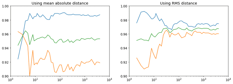
NoneYou'll have to excuse the lack of labels on the graph, as I've no idea how to add the labels at the moment. Blue is the percentage of sevens identified as not threes, orange is the percentage of threes identified as threes, and green is the average of the two. It looks like RMS is indeed better, but the interesting thing is that these stopped improving at around <100 samples.
I've exported the notebook to markdown and am using gatsby-remark-images for embedding images.


