// laurynasl
fast.ai Lesson 4
We're continuing with building a digit classifier. In the last post, we've created a simple classifier based on average pixel values for the numbers. Here, we'll actually use machine learning, because the algorithm will have parameters that we'll adjust based on how good it's doing it's job.
Let's start with reusing things from last session
from fastai.vision.all import *
from fastbook import *
import numpy as np
import matplotlib.pyplot as plt

matplotlib.rc('image', cmap='Greys')
path = untar_data(URLs.MNIST_SAMPLE)
Path.BASE_PATH = path
def image_tensors(purpose, digit):
images = (path/purpose/digit).ls().sorted()
tensors = [tensor(Image.open(im)) for im in images]
return torch.stack(tensors).float()/255
sevens = image_tensors('train', '7')
threes = image_tensors('train', '3')
sevens_valid = image_tensors('valid', '7')
threes_valid = image_tensors('valid', '3')First, we'll need to reshape the data, so that's it's faster to work with. We want to label each image with a 1 if it's a three and a 0 if it's a seven. We also want to simplify it into a vector of size 784 instead of a 28x28 matrix. We then zip these into a list. This part is a bit odd, as it seems quite ineffective, but later on, we'll use a data loader to turn an iterable of Tuple(x Tensor, y Tensor) into a mini batch tensor that will be used for calculations
train_x = torch.cat([threes, sevens]).view(-1, 28*28)
train_y = tensor([1]*len(threes) + [0]*len(sevens)).unsqueeze(-1)


train_dset= list(zip(train_x,train_y))
len(train_dset), train_dset[0][0].shape, train_dset[0][1].shape
(12396, torch.Size([784]), torch.Size([1]))Do the same for the validation dataset.
valid_x = torch.cat([threes_valid, sevens_valid]).view(-1, 28*28)
valid_y = tensor([1]*len(threes_valid) + [0]*len(sevens_valid)).unsqueeze(-1)


valid_dset = list(zip(valid_x,valid_y))
len(valid_dset), valid_dset[0][0].shape, valid_dset[0][1].shape
(2038, torch.Size([784]), torch.Size([1]))We'll be using a linear model with one parameter for each pixel. y = x * w + b. Let's initialize the weight and bias parameters with random values with standard deviation of 1.0.
def init_params(size): return torch.randn(size)

weights = init_params(28*28).requires_grad_()
bias = init_params(1).requires_grad_()
weights.shape, bias.shape
(torch.Size([784]), torch.Size([1]))Finally, let's define the parameterized function we'll be using.
def linear1(xb): return xb@weights + bias

preds = linear1(train_x)
preds
tensor([ -6.2330, -10.6388, -20.8865, ..., -15.9176, -1.6866, -11.3568], grad_fn=<AddBackward0>)Let's see how accurate it is right now (don't hold your breath yet.). We'll interpret a value above zero to indicate that the model predicts it to be a three and below or equal to 0 -- a seven.
((preds>0.0).float() == train_y).float().mean().item()0.5040026903152466~50 %. That's what you'd expect, as the paramets are all randomized.
Unfortunately, this function method won't work as a loss function, as it's changing in a stepwise manner. That is, when we change the paremeters slightly, the result might not change at all. That means the derivative will be zero and we won't change the parameter during our training loop. Let's define a better loss function here. This will use the sigmoid function to ensure that all predictions fall within the range of (0; 1) and the PyTorch where method to calculate how far the prediction was from the correct answer.
def mnist_loss(predictions, targets):
    predictions = predictions.sigmoid()
    return torch.where(targets==1, 1-predictions, predictions).mean()
Let's stuff the data into a DataLoader to load data in mini-batches, so that we don't need to loop in python land.
weights = init_params(28*28).requires_grad_()
bias = init_params(1).requires_grad_()

train_dl = DataLoader(train_dset, batch_size=256)
valid_dl = DataLoader(valid_dset, batch_size=256)

first(train_dl)[0].shape, first(train_dl)[1].shape
(torch.Size([256, 784]), torch.Size([256, 1]))Now we need to be able to calculate the gradients for each parameter. We do it by calling backwards after calculating a new value for the loss.
def calc_grad(xb, yb, model):
    preds = model(xb)
    loss = mnist_loss(preds, yb)
    loss.backward()

batch_x = train_x[:4]
batch_y = train_y[:4]

calc_grad(batch_x, batch_y, linear1)
weights.grad.mean(), bias.grad
(tensor(-5.9512e-08), tensor([-4.1723e-07]))To be honest, the mutable state baked into the gradient mechanism makes me cringe a bit, but I guess it's fine. I find it hard to keep track of all the mutations going on my head here.
Finally we can define a method to train our very simple neural net.
def train_epoch(model, lr, params):
    for xb,yb in train_dl:
        calc_grad(xb, yb, model)
        for p in params:
            p.data -= p.grad*lr
            p.grad.zero_()

def batch_accuracy(xb, yb):
    preds = xb.sigmoid()
    correct = (preds>0.5) == yb
    return correct.float().mean()

def validate_epoch(model):
    accs = [batch_accuracy(model(xb), yb) for xb,yb in valid_dl]
    return round(torch.stack(accs).mean().item(), 4)
And train it for some epochs and see what sort of results do we get
weights = init_params(28*28).requires_grad_()
bias = init_params(1).requires_grad_()

lr = 1.0
params = weights, bias
epochs = 40

accuracies = [validate_epoch(linear1)]
for i in range(epochs - 1):
    train_epoch(linear1, lr, params)
    accuracies.append(validate_epoch(linear1))

plt.axis([1, epochs, 0.9, 1])
plt.plot(range(epochs), accuracies)

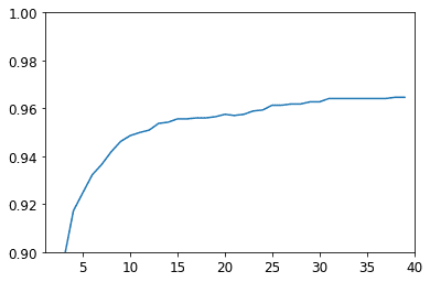
NoneWe see that we're in ballpark of the naive approach we took in the previous post. Not too impressive yet, this is the basis of stochastic gradient descent for use in machine learning.
We could extract the training function above into something a class, which is already provided by PyTorch. Instead we can just express everything we did up until now, using PyTorch utilities.
dls = DataLoaders(train_dl, valid_dl)

learn = Learner(dls,
                nn.Linear(28*28, 1),
                opt_func=SGD,
                loss_func=mnist_loss,
                metrics=batch_accuracy
)learn.fit(epochs, lr=lr)plt.axis([0, epochs, 0.9, 1])
plt.plot(range(epochs), accuracies, L(learn.recorder.values).itemgot(2))
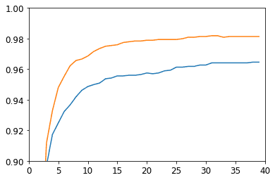
NoneOk, I'm confused here. It seems that either I messed something up in the dummy implementation or the PyTorch implmentation does a bit more under the hood. The PyTorch version looks more accurate
We can use this infrastructure to build even a better model by adding a non linearity between the layers. We need to do this because otherwise we just have a linear model with more parameters. We can do that by combining multiple layers like so:
simple_net = nn.Sequential(
    nn.Linear(28*28,30),
    nn.ReLU(),
    nn.Linear(30,1)
)

learn_sn = Learner(dls,
                   simple_net,
                   opt_func=SGD,
                   loss_func=mnist_loss,
                   metrics=batch_accuracy)

learn_sn.fit(epochs, 0.2)plt.axis([0, epochs, 0.9, 1])
plt.plot(range(epochs), list(zip(
accuracies,
L(learn.recorder.values).itemgot(2),
L(learn_sn.recorder.values).itemgot(2))))
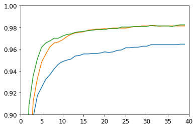
NoneIt looks like this more complex network was a bit faster to learn, however the overall accuracy did not change much.
Well here we have it. Machine learning.


